While using the Google sheet you must have dealt with a large number of data and there are chances that it would also have some duplicates. So to avoid the duplicates data you need to, first of all, identify them and then remove.
If the duplicate data is highlighted then it becomes much easier to see if there is nothing left out. It is a very difficult task if you try to see the duplicate figures and then remove them manually one by one.
Here, we will let you know about the basic steps to highlight and remove duplicates in Google Sheets.
The first thing that needs to be done is that the Google sheets should be open and then we will highlight the duplicate data.
Also Read: How to quickly factory reset your iMac like a pro?
How to highlight duplicate data in a single column in Google sheet

Step 1: Open the spreadsheet and select any column then go to the conditional formatting button that is available in the format rules section of the dropdown list.
Step 2: Now use the formula =countif(A1:A,A1)>1
Step 3: By using the above formula you can highlight the duplicate values as it will fill the colors of your choice.
Step 4: After completing the above steps, click on the done button and it will show all the highlighted duplicate values in a single column
You can repeat the same steps for other columns to get the highlighted duplicate values
Also Read: How to set up your D-link router and change password?
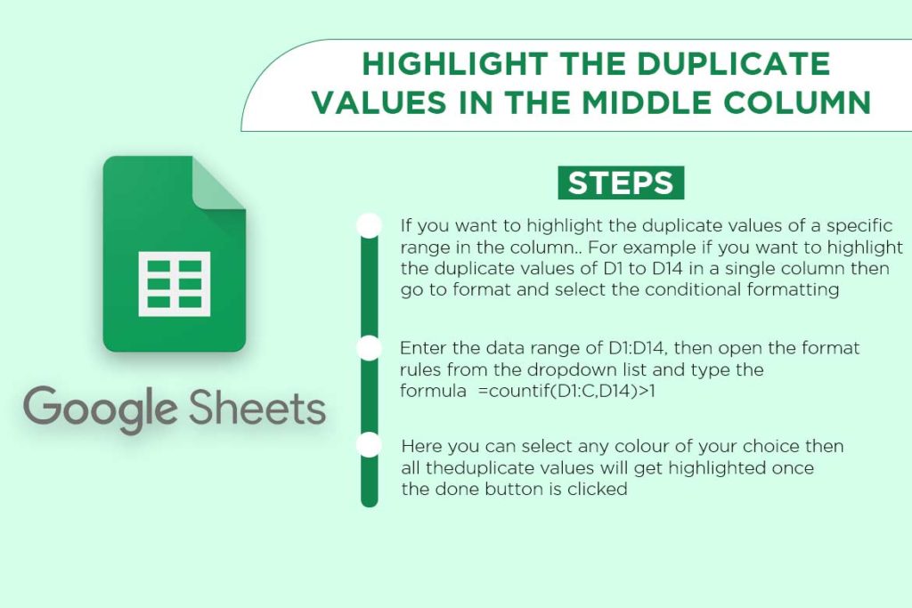
In case you want to highlight the duplicate values in the middle column in Google sheet

Step 1: If you want to highlight the duplicate values of a specific range in the column. For example, if you want to highlight the duplicate values of D1 to D14 in a single column then go to format and select the conditional formatting
Step 2: Enter the data range of D1:D14, then open the format rules from the dropdown list and type the formula =countif(D1:C,D14)>1
Step 3: Here you can select any colour of your choice then all the duplicate values will get highlighted once the done button is clicked
So far we have told you to highlight the duplicate values in a single and any other column but if you want to highlight the duplicate values in multiple columns then this is also very easy all you have to do is follow the below simple steps

Step 1: Open the Google Spreadsheet and select the multiple columns then select the range from B to F and press the format button
Step 2: Here you will have to click on the conditional formatting
Step 3: This is the time to use the formula which is very simple, Just type =countif(B1:E,F1)>1.
Step 4: Now select the colour of your choice and click on the done button, all the duplicate values in the selected columns will get highlighted
Now that we have told you about highlighting the duplicate values, it’s time to remove them.
Removing the highlighted duplicate values in Google Sheet is also a simple task all you have to do is follow the below simple steps
Step 1: Open the Google sheet and select the column in which duplicate values are available
Step 2: Click on the Data tab and use the remove duplicate option from the pop up
The above two steps can be used to remove duplicates from any columns in the Google sheet
Also Read: Microsoft Word: Learn to Transcribe or Dictate Audio With Word Online.


